$ \ifdefined\HCode % we are running tex4ht % don't load the physics package \require{physics} % \require{siunitx} \else % we are running LaTeX % \usepackage{physics} \fi \renewcommand{\phi}{\varphi} \renewcommand{\epsilon}{\varepsilon} \newcommand\define[1]{\textbf{#1}\index{#1}} % Letters/Font \DeclareMathOperator{\bF}{\mathbb{F}} \DeclareMathOperator{\bQ}{\mathbb{Q}} \DeclareMathOperator{\bZ}{\mathbb{Z}} \DeclareMathOperator{\bR}{\mathbb{R}} \DeclareMathOperator{\bC}{\mathbb{C}} \DeclareMathOperator{\bE}{\mathbb{E}} \DeclareMathOperator{\bN}{\mathbb{N}} \DeclareMathOperator{\bM}{\mathbb{M}} \DeclareMathOperator{\bH}{\mathbb{H}} \DeclareMathOperator{\bP}{\mathbb{P}} \DeclareMathOperator{\cH}{\mathcal{H}} \DeclareMathOperator{\cA}{\mathcal{A}} \DeclareMathOperator{\cB}{\mathcal{B}} \DeclareMathOperator{\cC}{\mathcal{C}} \newcommand\bb[1]{\mathbb{#1}} \newcommand\mc[1]{\mathcal{#1}} \newcommand{\w}[1]{\wedge#1} \newcommand\mean[1]{\bar{#1}} \newcommand\conj[1]{\bar{#1}} \DeclareMathOperator*{\argmin}{arg\,min} \DeclareMathOperator*{\argmax}{arg\,max} % Grouping Operators \newcommand{\floor}[1]{\left\lfloor#1\right\rfloor} \newcommand{\ceil}[1]{\left\lceil#1\right\rceil} \newcommand{\parens}[1]{\left(#1\right)} % note that we defined bracks not brace/braces because brace is already used by amsmath \newcommand{\bracks}[1]{\left\{#1\right\}} \newcommand{\sqbracks}[1]{\left[#1\right]} \newcommand{\clop}[1]{\left[#1\right)} \newcommand{\opcl}[1]{\left(#1\right]} \newcommand{\angles}[1]{\langle#1\rangle} \newcommand{\p}[1]{\left(#1\right)} % \newcommand{\b}[1]{\left\{#1\right\}} \newcommand{\q}[1]{\left[#1\right]} \newcommand{\abs}[1]{\left|#1\right|} \newcommand{\n}[1]{\left\lVert#1\right\rVert} % probability \DeclareMathOperator{\Cov}{Cov} \DeclareMathOperator{\Var}{Var} \DeclareMathOperator{\Cor}{Cor} \DeclareMathOperator{\median}{median} % https://tex.stackexchange.com/questions/154530/resolved-a-conditional-independence-symbol-that-looks-good-with-mid \newcommand{\ind}{\mathrel{\text{\scalebox{1.07}{$\perp\mkern-10mu\perp$}}}} % or \newcommand{\ind}{\perp\!\!\!\!\perp} % now included in the physics package %\newcommand{\norm}[1]{\left\lVert#1\right\rVert} \DeclareMathOperator{\Bias}{Bias} \DeclareMathOperator{\Range}{Range} % linear algebra \DeclareMathOperator{\nullity}{nullity} \DeclareMathOperator{\rowrank}{row rank} \DeclareMathOperator{\colrank}{column rank} % now in the physics package % \DeclareMathOperator{\tr}{Tr} % \DeclareMathOperator{\Tr}{Tr} \DeclareMathOperator{\perm}{perm} \DeclareMathOperator{\GL}{GL} \DeclareMathOperator{\SL}{SL} \DeclareMathOperator{\imm}{imm} \DeclareMathOperator{\poly}{poly} \DeclareMathOperator{\Lie}{Lie} \DeclareMathOperator{\Cl}{Cl} \DeclareMathOperator{\Span}{span} \DeclareMathOperator{\Int}{int} \DeclareMathOperator{\adj}{adj} % abstract algebra \DeclareMathOperator{\Aut}{Aut} \DeclareMathOperator{\id}{id} \DeclareMathOperator{\Id}{Id} \DeclareMathOperator{\Inn}{Inn} \DeclareMathOperator{\irr}{irr} \DeclareMathOperator{\Frac}{Frac} \DeclareMathOperator{\Frob}{Frob} % category theory \DeclareMathOperator{\ob}{ob} \DeclareMathOperator{\Set}{Set} \DeclareMathOperator{\Grp}{Grp} \DeclareMathOperator{\Ring}{Ring} \DeclareMathOperator{\Top}{Top} \DeclareMathOperator{\Vect}{Vect} \DeclareMathOperator{\End}{End} \DeclareMathOperator{\Hom}{Hom} \DeclareMathOperator{\im}{im} % \DeclareMathOperator{\Vec}{Vec} \DeclareMathOperator{\Rel}{Rel} \DeclareMathOperator{\Mon}{Mon} \DeclareMathOperator{\Pre}{Pre} \DeclareMathOperator{\SRel}{SRel} \DeclareMathOperator{\Ab}{Ab} \DeclareMathOperator{\Perm}{Perm} \DeclareMathOperator{\Nat}{Nat} \DeclareMathOperator{\Cat}{Cat} % now in physics package % \DeclareMathOperator{\op}{op} \DeclareMathOperator{\FinStoch}{FinStoch} \DeclareMathOperator{\Stoch}{Stoch} % number theory \DeclareMathOperator{\rad}{rad} \DeclareMathOperator{\Disc}{Disc} \DeclareMathOperator{\res}{res} \DeclareMathOperator{\lcm}{lcm} % differential geometry \DeclareMathOperator{\Man}{Man} \DeclareMathOperator{\supp}{supp} \DeclareMathOperator{\Diff}{Diff} \DeclareMathOperator{\VB}{VB} % complexity theory \DeclareMathOperator{\fspace}{FSPACE} \DeclareMathOperator{\sspace}{SPACE} \DeclareMathOperator{\pspace}{PSPACE} \DeclareMathOperator{\AR}{AR} \DeclareMathOperator{\MA}{MA} \DeclareMathOperator{\B}{B} \DeclareMathOperator{\ARMA}{ARMA} \DeclareMathOperator{\diag}{diag} \DeclareMathOperator{\IMA}{IMA} \DeclareMathOperator{\ARIMA}{ARIMA} \DeclareMathOperator{\Vol}{Vol} \DeclareMathOperator{\essup}{essup} \DeclareMathOperator{\essinf}{essinf} \DeclareMathOperator{\Bernoulli}{Bernoulli} \DeclareMathOperator{\Law}{Law} \DeclareMathOperator{\Normal}{Normal} \DeclareMathOperator{\Geometric}{Geometric} \DeclareMathOperator{\Poisson}{Poisson} \DeclareMathOperator{\Uniform}{Uniform} \DeclareMathOperator{\Beta}{Beta} \DeclareMathOperator{\TV}{TV} \DeclareMathOperator{\io}{i.o.} \DeclareMathOperator{\ale}{a.e.} \DeclareMathOperator{\as}{a.s.} \DeclareMathOperator{\iid}{i.i.d.} % least fixed point \DeclareMathOperator{\lfp}{lfp} \DeclareMathOperator{\sign}{sign} \DeclareMathOperator{\pval}{p.v.} \DeclareMathOperator{\sgn}{sgn} \DeclareMathOperator{\dom}{dom} \DeclareMathOperator{\Ran}{Ran} \DeclareMathOperator{\Hol}{Hol} \DeclareMathOperator{\cl}{cl} \DeclareMathOperator{\Pol}{Pol} \DeclareMathOperator{\sinc}{sinc} \DeclareMathOperator{\E}{\mathbb{E}} \DeclareMathOperator{\Pr}{\mathbb{P}} \DeclareMathOperator{\R}{\mathbb{R}} $

Simple Markov, Chebyshev, and Hoeffding Inequalities

Published: 28 Feb 2025

Last updated: 29 Mar 2025

Categories Tags

Here are simple visuals for the Markov, Chebyshev, and Chernoff inequalities, as well as a connection to Cramer’s theorem and intuition about how to derive the Hoeffding inequality from them.

Markov, Chebyshev, and Chernoff

Let $X$ be a random variable. Using an indicator variable, we have $\Pr\sqbracks{\abs{X-c}\geq a}=\E\sqbracks{𝟙_{\abs{X-c}\geq a}}$. We can recover various bounds/inequalities by considering different values of $c$ and functions $f(x)$ that dominate $𝟙_{|x-c|\geq a}$. By the monotonicity of the Lebesgue integral, we have that $\E[𝟙_{|X-c|\geq a}]\leq \E[f(X)]$.
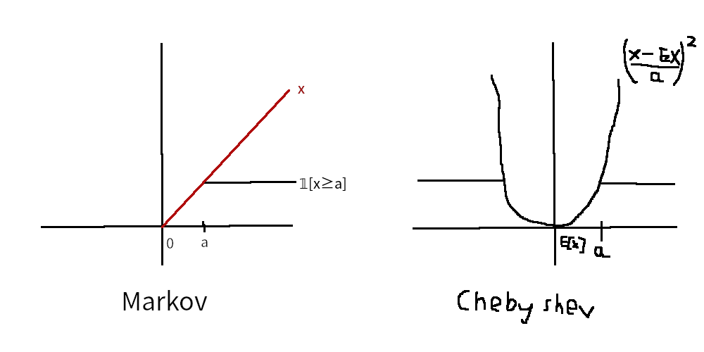
If $c=0$, $f(x)=x/a$, and $X$ is nonnegative, then we get Markov’s inequality as

\[\Pr[X\geq a]=\E[𝟙_{X\geq a}]\leq\E[X/a]=\E[X]/a\]

If $c=\E[X]$ and $f(x)=((x-\E[X])/a)^2$ (the quadratic that passes through $(\E[X]+a,1)$), then we get Chebyshev’s inequality as

\[\Pr[\abs{X-\E[X]}\geq a]=\E[𝟙_{\abs{X-\E[X]}\geq a}]\leq\E[((X-\E[X])/a)^2]=\Var[X]/a^2\]

With $c=0$ and $f(x)=\phi(x)/\phi(a)$ for $\phi$ nondecreasing and $X$ nonnegative, we get extensions of Markov’s inequality,

\[\Pr[X\geq a]\leq\E[\phi(X)]/\phi(a)\]

For example, with $\phi(x)=e^{tx}$, we get the Chernoff bound

\[\Pr[X\geq a]\leq M[t]e^{-ta}\]

where $M[t]$ is the moment generating function.

Hoeffding bound and connection to Cramer’s theorem

As an extension of Chernoff’s bound, with $Y_i$ iid and $X=S_n=∑_i(Y_i-𝔼[Y_i])$, we instead get

\[\Pr[X\geq a]\leq M_{X}[t]e^{-ta}=M_{\sum_iY_i}[t]e^{-ta}=\prod_i M_{Y}[t]e^{-ta}=M_Y[t]^ne^{-ta}=e^{n\ln M_Y[t]-ta}\]

where $μ(t)=\log M(t)$. This bound (or the variant where we look at the average $\bar{Y}_n=X/n$ to get $\Pr[\bar{Y}_n\geq a]≤e^{-n(ta-μ(t)}$) is useful for thinking about Cramer’s theorem.

We can prove the Hoeffding inequality from this. First, we need the following lemma: For $X$ a random variable with $a≤X≤b$, for any $t∈ℝ$, $\ln M(t)≤t𝔼[X]+t^2(b-a)^2/8$. We can think of this as being related to the Taylor series of $e^{tX}$; $e^{tX}=1+tX+t^2X^2/2!+…$ so $𝔼[e^{tX}]=1+t𝔼[X]+t^2𝔼[X^2]/2!+…$, and taking $\ln$ of both sides, we get

\[\begin{align*} \ln \mathbb{E}[e^{tX}] &= \ln(1 + t\mathbb{E}[X] + \frac{t^2\mathbb{E}[X^2]}{2!} + O(t^3)) \\ &= (t\mathbb{E}[X] + \frac{t^2\mathbb{E}[X^2]}{2!} + O(t^3)) - \frac{1}{2}(t\mathbb{E}[X] + \frac{t^2\mathbb{E}[X^2]}{2!} + O(t^3))^2 + O(t^3) \\ &= t\mathbb{E}[X] + \frac{t^2}{2}(\mathbb{E}[X^2] - \mathbb{E}[X]^2) + O(t^3) \end{align*}\]

using the Taylor series $\ln(1+x)=x-x^2/2+…$. This explains where the linear term comes from, and if we look at the quadratic term, we find an intuitive but nonrigorous way to get $8$. We have

\[\frac{t^2}{2}(𝔼[X^2]-𝔼[X]^2)=\frac{t^2}{2}\Var(X)\]

and using Popoviciu’s inequality on variances, we know that $\Var(X)\leq (b-a)^2/4$, so overall the quadratic terms are bounded by $(b-a)^2/8$. The fact that higher order terms can also be contained in this bound, and that they give an upper bound is where handwaving comes in. The proof is just a simple optimization problem, but I don’t have any more intuition about it.

From this, we can derive Hoeffding’s inequality by applying the lemma and minimizing the bound in $t$:

\[\Pr[X\geq ε] \leq e^{n\ln M_Y[t]-tε} \leq e^{nt^2(b-a)^2/8-tε}\]

We differentiate the exponent with respect to $t$:

\[\frac{d}{dt}(nt^2(b-a)^2/8-tε) = \frac{n(b-a)^2t}{4}-ε\]

Setting this equal to 0, we get $\frac{n(b-a)^2t}{4}=ε$ or $t = \frac{4ε}{n(b-a)^2}$. Then plugging this back in, we have

\[\Pr[X\geq ε] \leq \exp\left(\frac{n(b-a)^2}{8}\cdot\frac{16ε^2}{n^2(b-a)^4}-ε\cdot\frac{4ε}{n(b-a)^2}\right) = \exp\left(\frac{2ε^2}{n(b-a)^2}-\frac{4ε^2}{n(b-a)^2}\right) = \exp\left(-\frac{2ε^2}{n(b-a)^2}\right)\]

which is the Hoeffding inequality!

An easy generalization of this (which is what is usually listed as the full Hoeffding inequality) is allowing $Y_i$ to have different bounds $(a_i,b_i)$; in that case, the denominator changes to $∑_i(b_i-a_i)^2$.

Sources